You should know now:

• the basic concept of analysis of variance
• the usage of the command lm() for analysis of variance
• that y ~ x in R mean y dependent on x (formula syntax)
• how the visualize anova using boxplots

• load the babies data set using read_excel():
  
• the column wt contains the birth weight in ounces; add another column bwt containing the birth weight in kg

• do an one-way anova of birth weight dependent on

  • 1. race (mother's race)
  • 2. smoke (mother's smoking status)
  • 3. number (number of cigs smoked per day)

• What are the percentages of explained variance in each model?

• Taken separately, which of the three variables explained most of the variance of birth weight?

• What is the mean birth weight of race mex?

• Which level of each of the three predictors has the lowest (resp. highest) mean birth weight?

• Visualize using ggplot2!

library(readxl)
babies <- read_excel("session6dta/babies.xlsx",1)
babies$bwt <- babies$wt/35.274
m1 <- lm(bwt ~ race, data = babies)
m2 <- lm(bwt ~ factor(smoke), data = babies)
m3 <- lm(bwt ~ number, data = babies)

summary(m1)

## 
## Call:
## lm(formula = bwt ~ race, data = babies)
## 
## Residuals:
##      Min       1Q   Median       3Q      Max 
## -1.66245 -0.30168  0.01017  0.32201  1.72258 
## 
## Coefficients:
##             Estimate Std. Error t value Pr(>|t|)    
## (Intercept)  3.13069    0.07640  40.977  < 2e-16 ***
## raceblack    0.07955    0.08300   0.958  0.33809    
## racemex      0.38890    0.11072   3.513  0.00046 ***
## racemixed    0.26558    0.12693   2.092  0.03661 *  
## raceunknown  0.75319    0.51251   1.470  0.14193    
## racewhite    0.31779    0.07831   4.058 5.26e-05 ***
## ---
## Signif. codes:  0 '***' 0.001 '**' 0.01 '*' 0.05 '.' 0.1 ' ' 1
## 
## Residual standard error: 0.5068 on 1218 degrees of freedom
##   (12 observations deleted due to missingness)
## Multiple R-squared:  0.04498,    Adjusted R-squared:  0.04106 
## F-statistic: 11.47 on 5 and 1218 DF,  p-value: 7.661e-11

summary(m1)$r.squared

## [1] 0.04497971

summary(m1)$r.squared

## [1] 0.04497971

summary(m2)$r.squared

## [1] 0.05879809

summary(m3)$r.squared

## [1] 0.04663428

library(ggplot2)
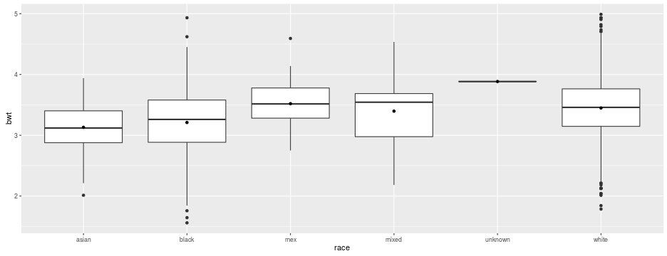
ggplot(babies, aes(x = race, y = bwt)) +
  geom_boxplot() +
  stat_summary(geom = "point", fun.y = "mean")

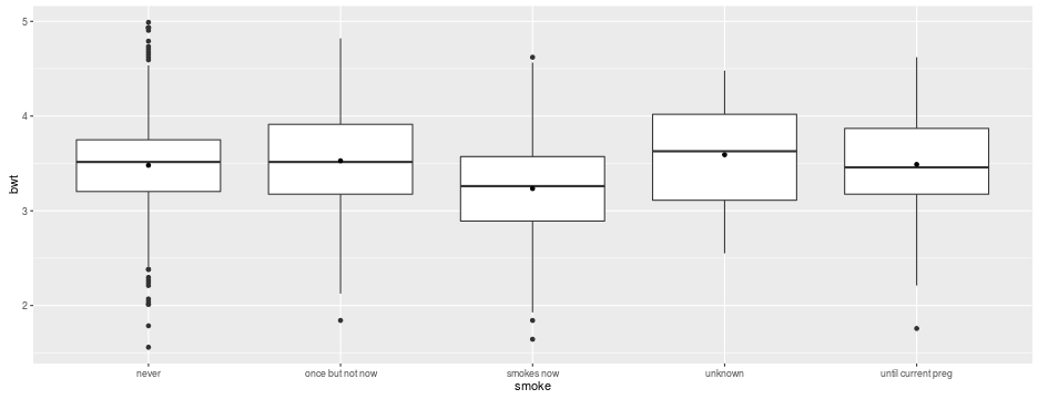
ggplot(babies, aes(x = smoke, y = bwt)) +
  geom_boxplot() +
  stat_summary(geom = "point", fun.y = "mean")

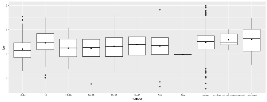
ggplot(babies, aes(x = number, y = bwt)) +
  geom_boxplot() +
  stat_summary(geom = "point", fun.y = "mean")

coef(summary(m1))

##               Estimate Std. Error    t value      Pr(>|t|)
## (Intercept) 3.13068601 0.07640112 40.9769674 1.993267e-231
## raceblack   0.07954547 0.08300438  0.9583285  3.380873e-01
## racemex     0.38890349 0.11071573  3.5126307  4.599375e-04
## racemixed   0.26558320 0.12692707  2.0924079  3.660861e-02
## raceunknown 0.75319447 0.51251426  1.4696069  1.419265e-01
## racewhite   0.31778537 0.07830927  4.0580812  5.262889e-05

• install (if not already done) and load the package granovaGG
  
• the following code produces a graphical representation of an anova analysis
• try to understand the different components

library(granovaGG)
granovagg.1w(babies$bwt,babies$smoke)

• there are different situation where it is advisable to recode variables e.g.
  • some characteristic is coded in numbers but a level/label combination would be more appropriate
  • one want to change a existing coding e.g. ja/nein to yes/no
  • missing values are coded as numbers and we want to transform them into real missings

• a factor is a vector that contain only predefined values
• it is used to store categorical data
• the levels()-label combination of a factor defines the set of allowed values

table(babies$sex)

## 
##   0   1 
## 626 610

class(babies$sex)

## [1] "numeric"

babies$sex.mf <- factor(babies$sex, 
                        levels = c(0,1),
                        labels = c("male","female"))
class(babies$sex.mf)

## [1] "factor"

table(babies$sex.mf)

## 
##   male female 
##    626    610

• use factor() to change the marital and inc variable from numeric to factor
  • 1 = married, 2 = legally separated, 3 = divorced, 4 = widowed, 5 = never married
  • 0 = <2500, 1 = 2500-4999, 2 = 5000-7499, 3 = 7500-9999, ..., 9 = 15000+, 98 = unknown, 99 = not asked
• table the two variables using table() and prop.table(); what is the percentage of <2500 amongst married and what amongst never married?

babies$marital <- factor(babies$marital, 
                         levels = 1:5, 
                         labels = c("married","legally separated",
                                    "divorced","widowed","never married"))
babies$inc <- factor(babies$inc,
                     levels = c(0:9,98,99),
                     labels = c("<2500",
                                paste(seq(2500,20000,by = 2500),
                                      seq(4999,22500,by = 2500),sep = "-"),
                                "25000+","unknown","not asked"))

addmargins(prop.table(table(babies$inc,babies$marital),2))

##              
##                  married legally separated   divorced widowed
##   <2500       0.02400662        0.06666667 0.00000000        
##   2500-4999   0.15397351        0.26666667 0.40000000        
##   5000-7499   0.14486755        0.06666667 0.20000000        
##   7500-9999   0.14900662        0.00000000 0.00000000        
##   10000-12499 0.11341060        0.06666667 0.00000000        
##   12500-14999 0.10264901        0.13333333 0.00000000        
##   15000-17499 0.05877483        0.06666667 0.00000000        
##   17500-19999 0.11672185        0.06666667 0.20000000        
##   20000-22499 0.02069536        0.00000000 0.00000000        
##   25000+      0.01738411        0.06666667 0.20000000        
##   unknown     0.09850993        0.20000000 0.00000000        
##   not asked   0.00000000        0.00000000 0.00000000        
##   Sum         1.00000000        1.00000000 1.00000000        
##              
##               never married Sum
##   <2500          0.16666667    
##   2500-4999      0.50000000    
##   5000-7499      0.00000000    
##   7500-9999      0.00000000    
##   10000-12499    0.00000000    
##   12500-14999    0.00000000    
##   15000-17499    0.00000000    
##   17500-19999    0.00000000    
##   20000-22499    0.00000000    
##   25000+         0.00000000    
##   unknown        0.33333333    
##   not asked      0.00000000    
##   Sum            1.00000000

babies$sex.jm <- factor(babies$sex.mf, 
                        levels = c("male","female"),
                        labels = c("Junge","Maedchen"))
table(babies$sex.jm)

## 
##    Junge Maedchen 
##        0     1236

• another kind of issue is a problem like the following:
• the drace variable contains 11+ races plus one unknown coding
• coding 0-5 means all white, 6 mex, 7 black, 8 asian, 9 and 10 mixed, 99 unknown

library(car)
babies$drace <- recode(babies$drace,
                       '0:5="white";6="mex";7="black";
                       8="asian";c(9,10)="mixed";99=NA')

• use the variables race and drace to get the percentage of mixed paires (man and woman from different races)

prop.table(table(babies$race == babies$drace))

## 
##      FALSE       TRUE 
## 0.05660377 0.94339623